Forward and Futures Contracts

import numpy as np
import matplotlib.pyplot as plt

# Set random seed for reproducibility
np.random.seed(42)

# Configure plotting style
plt.style.use('ggplot')
plt.rcParams['figure.figsize'] = [12, 6]
plt.rcParams['font.size'] = 12

Introduction

Forward and futures contracts are fundamental derivatives in financial markets. While they serve similar purposes, they have important differences in their structure and trading mechanisms.

Forward Contracts

A forward contract is a customized agreement between two parties to buy or sell an asset at a specified future date for a price agreed upon today. Key characteristics:

1. Private Agreement:
   • Traded over-the-counter (OTC)
   • Customized terms
   • No intermediary
2. Settlement:
   • Single payment at maturity
   • Physical or cash settlement
   • No intermediate cash flows
3. Counterparty Risk:
   • No guarantee mechanism
   • Credit risk is a concern
   • Default risk must be considered

Futures Contracts

A futures contract is a standardized agreement traded on exchanges. Key characteristics:

1. Exchange-Traded:
   • Standardized terms
   • Highly liquid
   • Price transparency
2. Settlement:
   • Daily marking-to-market
   • Margin requirements
   • Clearinghouse guarantee
3. Risk Management:
   • Minimal counterparty risk
   • Regular margin adjustments
   • Exchange oversight

Understanding Cost of Carry

The cost of carry is a fundamental concept in forward and futures pricing. It represents the net cost of holding an asset over time. Let’s break this down with a practical example.

Example: Agricultural Commodities

Consider a wheat farmer and a flour mill:

1. Immediate Purchase (Spot Market):
   • Buy wheat today at spot price
   • Pay for storage
   • Pay for insurance
   • Incur financing costs
   • Risk of quality deterioration
2. Forward Contract:
   • Lock in price today
   • Delivery in 6 months
   • Seller bears storage costs
   • No immediate capital outlay
   • Quality guaranteed at delivery

Components of Cost of Carry

1. Storage Costs:
   • Physical storage space
   • Handling and maintenance
   • Insurance
2. Financing Costs:
   • Interest on borrowed funds
   • Opportunity cost of capital
3. Benefits of Holding:
   • Convenience yield
   • Income (e.g., dividends)
   • Quality optionality

def calculate_forward_price(S0, r, q, T, dividends=None):
    """
    Calculate forward price using the cost of carry model.
    
    Parameters:
    -----------
    S0 : float
        Spot price
    r : float
        Risk-free rate (annualized)
    q : float
        Convenience yield or dividend yield (annualized)
    T : float
        Time to maturity in years
    dividends : list of tuples, optional
        List of (amount, time) tuples for discrete dividends
        
    Returns:
    --------
    float
        Forward price
    """
    # Basic forward price without dividends
    F = S0 * np.exp((r - q) * T)
    
    # Adjust for discrete dividends if provided
    if dividends:
        for D, t in dividends:
            F -= D * np.exp(r * (T - t))
            
    return F

# Example parameters
S0 = 100  # Spot price
r = 0.05  # Risk-free rate (5%)
q = 0.02  # Convenience yield (2%)
T = 1.0   # One year to maturity

# Calculate forward price without dividends
F_no_div = calculate_forward_price(S0, r, q, T)

# Calculate with some discrete dividends
dividends = [(2.0, 0.25), (2.0, 0.75)]  # $2 dividend at 3 months and 9 months
F_with_div = calculate_forward_price(S0, r, q, T, dividends)

print(f"Forward Price (No Dividends): ${F_no_div:.2f}")
print(f"Forward Price (With Dividends): ${F_with_div:.2f}")

# Plot forward prices for different maturities
T_range = np.linspace(0, 2, 100)
F_range_no_div = [calculate_forward_price(S0, r, q, t) for t in T_range]
F_range_with_div = [calculate_forward_price(S0, r, q, t, dividends) for t in T_range]

plt.figure(figsize=(12, 6))
plt.plot(T_range, F_range_no_div, label='No Dividends', linewidth=2)
plt.plot(T_range, F_range_with_div, label='With Dividends', linewidth=2)
plt.axhline(y=S0, color='k', linestyle='--', label='Spot Price')

plt.title('Forward Prices vs Time to Maturity')
plt.xlabel('Time to Maturity (Years)')
plt.ylabel('Forward Price ($)')
plt.legend()
plt.grid(True)
plt.show()

Forward Price (No Dividends): $103.05
Forward Price (With Dividends): $98.94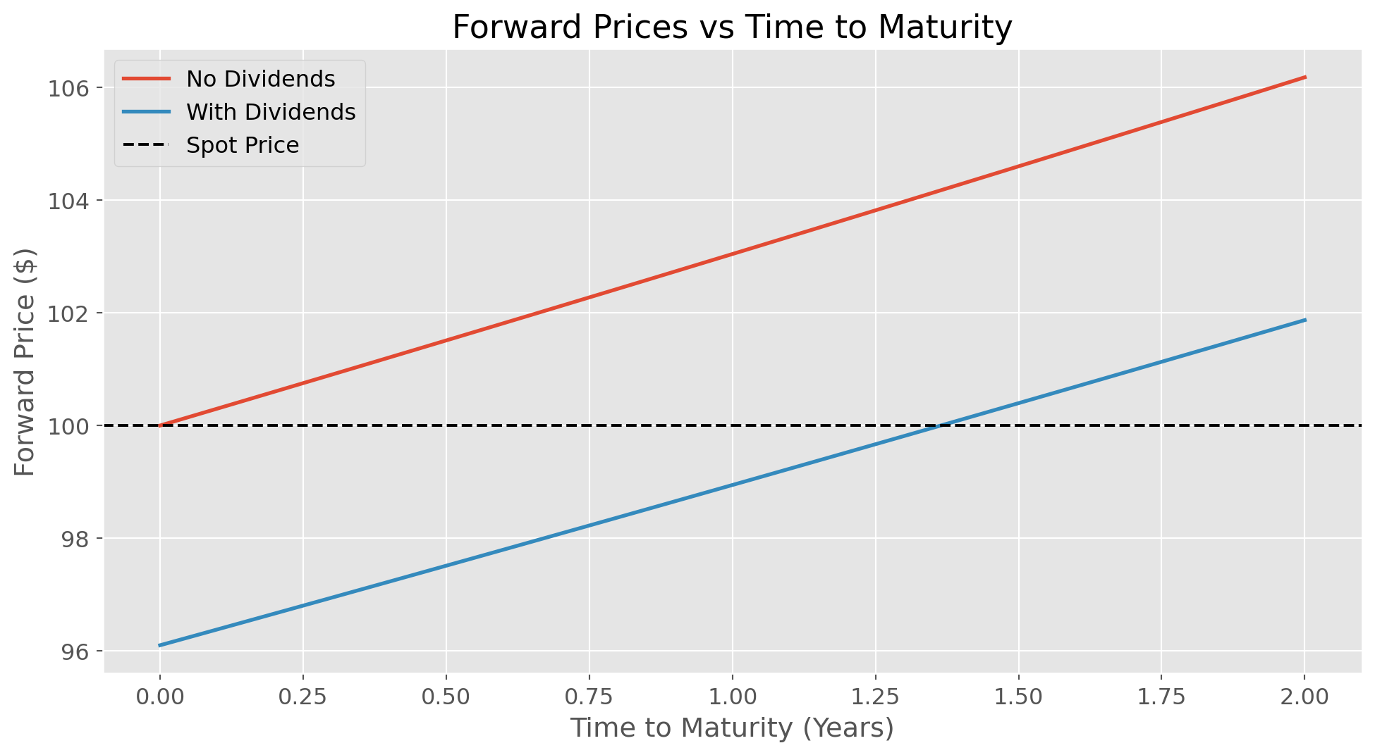

Forward Price Formula and Its Components

The forward price formula is derived from the principle of no-arbitrage and incorporates several key components:

Basic Formula

The forward price \(F\) for an asset with spot price \(S_0\) is given by:

\[F = S_0 e^{(r-q)T} - \sum_{i=1}^N D_i e^{r(T-t_i)}\]

where: - \(F\) is the forward price to be paid at time \(T\) - \(S_0\) is the current spot price - \(r\) is the risk-free interest rate (continuous compounding) - \(q\) is the continuous dividend yield or convenience yield - \(T\) is the time to maturity in years - \(D_i\) is a discrete dividend paid at time \(t_i\) where \(0 < t_i < T\)

Key Components Explained

1. Spot Price (\(S_0\)):
   • Current market price of the asset
   • Starting point for forward pricing
2. Risk-Free Rate (\(r\)):
   • Opportunity cost of funds
   • Usually based on government securities
   • Assumed to be constant for simplicity
3. Dividend/Convenience Yield (\(q\)):
   • Continuous yield from holding the asset
   • For stocks: dividend yield
   • For commodities: convenience yield
4. Time Factor (\(T\)):
   • Time to maturity in years
   • Affects the compounding of carrying costs
5. Discrete Dividends (\(D_i\)):
   • Known dividend payments
   • Adjusted for time value of money
   • Reduces the forward price

def analyze_forward_price_sensitivity(S0=100, r=0.05, q=0.02, T=1.0, dividends=None):
    """
    Analyze how forward prices change with different parameters.
    
    Parameters are same as calculate_forward_price function.
    """
    # Parameter ranges
    r_range = np.linspace(0, 0.1, 50)  # 0% to 10%
    q_range = np.linspace(0, 0.1, 50)  # 0% to 10%
    S0_range = np.linspace(50, 150, 50)  # $50 to $150
    
    # Calculate sensitivity to interest rates
    F_r = [calculate_forward_price(S0, r_i, q, T, dividends) for r_i in r_range]
    
    # Calculate sensitivity to convenience yield
    F_q = [calculate_forward_price(S0, r, q_i, T, dividends) for q_i in q_range]
    
    # Calculate sensitivity to spot price
    F_S0 = [calculate_forward_price(S0_i, r, q, T, dividends) for S0_i in S0_range]
    
    # Create subplots
    fig, (ax1, ax2, ax3) = plt.subplots(1, 3, figsize=(18, 5))
    
    # Plot sensitivity to interest rate
    ax1.plot(r_range * 100, F_r, 'b-', linewidth=2)
    ax1.set_title('Forward Price vs Interest Rate')
    ax1.set_xlabel('Interest Rate (%)')
    ax1.set_ylabel('Forward Price ($)')
    ax1.grid(True)
    
    # Plot sensitivity to convenience yield
    ax2.plot(q_range * 100, F_q, 'g-', linewidth=2)
    ax2.set_title('Forward Price vs Convenience Yield')
    ax2.set_xlabel('Convenience Yield (%)')
    ax2.set_ylabel('Forward Price ($)')
    ax2.grid(True)
    
    # Plot sensitivity to spot price
    ax3.plot(S0_range, F_S0, 'r-', linewidth=2)
    ax3.plot(S0_range, S0_range, 'k--', label='Spot Price')
    ax3.set_title('Forward Price vs Spot Price')
    ax3.set_xlabel('Spot Price ($)')
    ax3.set_ylabel('Forward Price ($)')
    ax3.legend()
    ax3.grid(True)
    
    plt.tight_layout()
    plt.show()

# Run sensitivity analysis
print("Analyzing Forward Price Sensitivity to Various Parameters...")
analyze_forward_price_sensitivity()

Analyzing Forward Price Sensitivity to Various Parameters...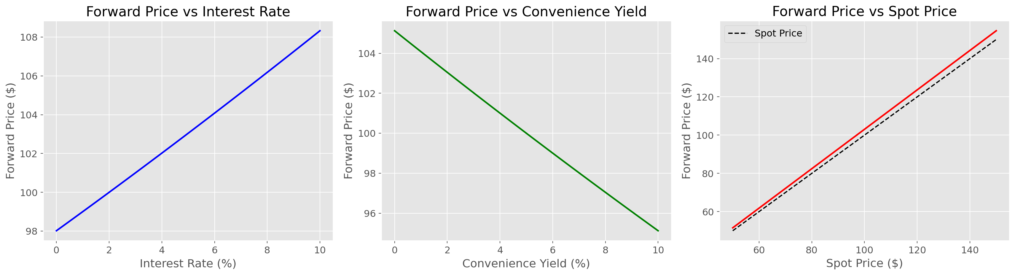

def simulate_futures_margin(S0=100, mu=0.1, sigma=0.2, T=1.0, n_steps=252, n_paths=5):
    """
    Simulate futures margin calls using geometric Brownian motion for the underlying.
    
    Parameters:
    -----------
    S0 : float
        Initial spot price
    mu : float
        Drift rate (annualized)
    sigma : float
        Volatility (annualized)
    T : float
        Time to maturity in years
    n_steps : int
        Number of time steps (trading days)
    n_paths : int
        Number of paths to simulate
    """
    # Time grid
    dt = T/n_steps
    t = np.linspace(0, T, n_steps)
    
    # Initialize arrays
    S = np.zeros((n_paths, n_steps))
    S[:, 0] = S0
    
    # Simulate price paths
    for i in range(n_paths):
        for j in range(1, n_steps):
            dW = np.sqrt(dt) * np.random.normal()
            S[i, j] = S[i, j-1] * np.exp((mu - 0.5*sigma**2)*dt + sigma*dW)
    
    # Calculate daily margin calls
    margin_calls = np.diff(S, axis=1)
    
    # Plot results
    plt.figure(figsize=(12, 8))
    
    # Plot price paths
    plt.subplot(2, 1, 1)
    for i in range(n_paths):
        plt.plot(t, S[i], label=f'Path {i+1}')
    plt.title('Simulated Price Paths')
    plt.xlabel('Time (years)')
    plt.ylabel('Price ($)')
    plt.legend()
    plt.grid(True)
    
    # Plot margin calls
    plt.subplot(2, 1, 2)
    for i in range(n_paths):
        plt.plot(t[1:], margin_calls[i], label=f'Path {i+1}')
    plt.title('Daily Margin Calls')
    plt.xlabel('Time (years)')
    plt.ylabel('Margin Call ($)')
    plt.axhline(y=0, color='k', linestyle='--')
    plt.legend()
    plt.grid(True)
    
    plt.tight_layout()
    plt.show()
    
    # Print summary statistics
    print("\nMargin Call Statistics:")
    print(f"Average Daily Margin Call: ${np.mean(margin_calls):.2f}")
    print(f"Max Positive Margin Call: ${np.max(margin_calls):.2f}")
    print(f"Max Negative Margin Call: ${np.min(margin_calls):.2f}")
    print(f"Standard Deviation: ${np.std(margin_calls):.2f}")

# Run simulation
print("Simulating Futures Margin Calls...")
simulate_futures_margin()

Simulating Futures Margin Calls...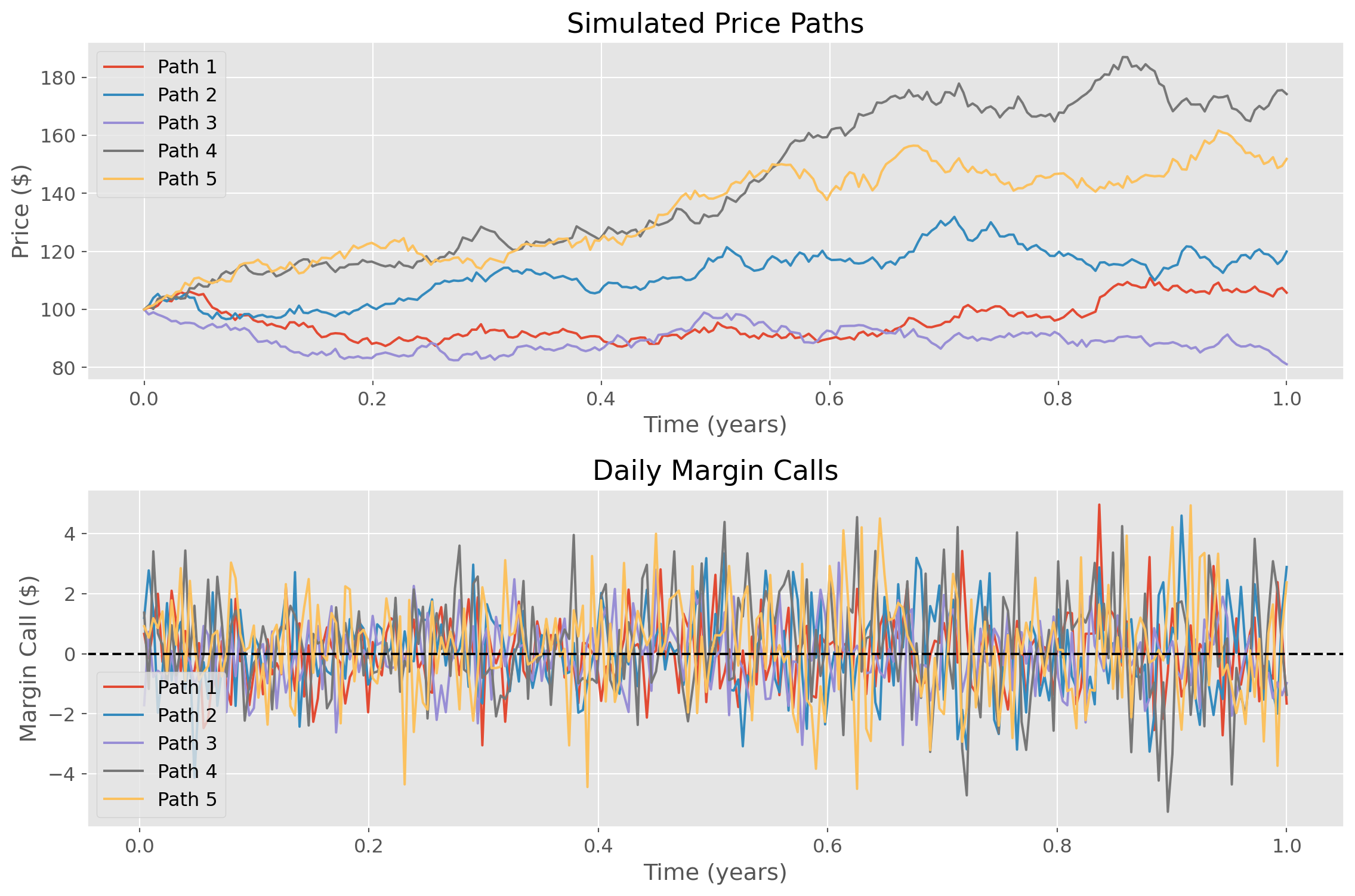

Margin Call Statistics:
Average Daily Margin Call: $0.11
Max Positive Margin Call: $4.97
Max Negative Margin Call: $-5.27
Standard Deviation: $1.48